Formula
The operation is indicated by an asterisk. The convolution of two functions is equal to the product of the two functions integrated. Since images are composed of pixels, functions are discrete when processing images.
Convolution of two functions:
$ f(x) * g(x) = \displaystyle\int_{-\infty}^{\infty} f(\tau) ⋅ g(x - \tau) \, d\tau $
Visualisation
The process of convolution can be thought of as one function sliding over the other, and at each point the result is the integral of the product of overlapping values, or the sum in the case of discrete convolution.
Guaussian blur
A Gaussian kernel can be used to smooth a function. This can be good for noise, but information may be lost in the process. A rectangular kernel also smoothes, but might give an abnormal, chunky result for images.
2D Convolution
The formula can be extended to two dimensions to convolve images. The kernel slides through the image changing the values of each pixel based on its neigbourhood of a given size.
$ f(x, y) * g(x, y) = \displaystyle\iint_{-\infty}^{\infty} f(\tau, \mu) ⋅ g(x - \tau, y - \mu) \, d\tau d\mu $

*
=

Properties
Convolution is commutative and associative, so for example an operation using a symmetric Gaussian 2D kernel can be split into 2 consecutive one-dimensional convolutions, reducing the number of operations.
$ f * g = g * f $
$ (f * g) * h = f * (g * h) $
Feature extraction
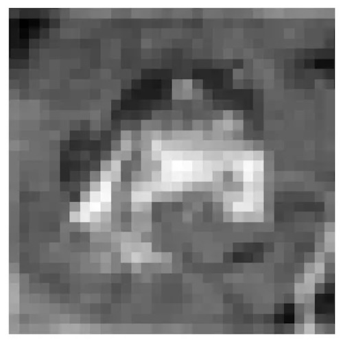
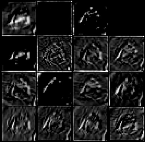
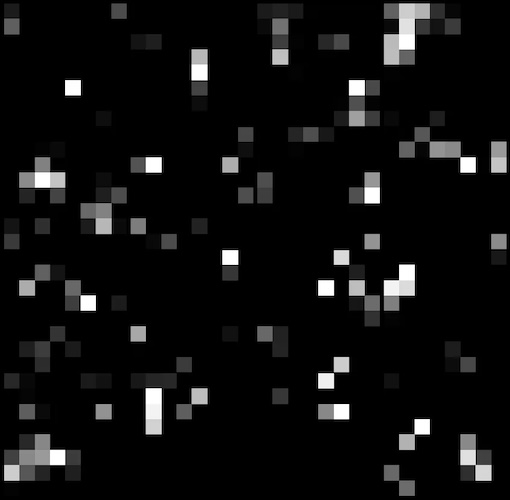
Convolutional Neural Networks (CNNs) form their own kernels to extract features from images when they are training on a given dataset. The neural network usually trains on the output of multiple convolutional layers.
# Rodrigo Silva: Exploring Feature Extraction with CNNs, Towards Data Science
#
https://towardsdatascience.com/exploring-feature-extraction-with-cnns-345125cefc9a
Fourier transform
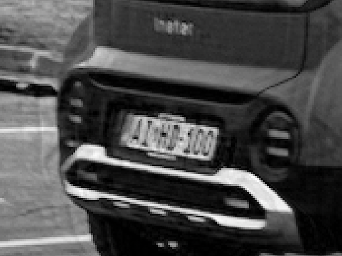
Just like a function, a photo can be converted into frequency domain. The convolution operation becomes a simple multiplication in frequency domain, so by applying the FFT algorithm to both the image and kernel and then multiplying them together, convolution is achieved. After converting back (IFFT), the result is the same as in the spatial domain by sliding the filter through. The really useful feature of this method, besides its speed, is that it can be done backwards. Deconvolution is simply a division in frequency domain, and by estimating kernels, the reconstruction of poor quality or blurred photographs is feasible.
$ f(x, y) * g(x, y) = F(u, v) ⋅ G(u, v) $